Molecular dynamics simulations of bulk water#
In this example, we show how to perform molecular dynamics of bulk water using the popular interatomic TIP3P potential (W. L. Jorgensen et. al.) and LAMMPS.
import numpy as np

%matplotlib inline
import matplotlib.pylab as plt
from pyiron_atomistics import Project
import ase.units as units
import pandas
pr = Project("tip3p_water")
Creating the initial structure#
We will setup a cubic simulation box consisting of 27 water molecules density density is 1 g/cm\(^3\). The target density is achieved by determining the required size of the simulation cell and repeating it in all three spatial dimensions
density = 1.0e-24  # g/A^3
n_mols = 27
mol_mass_water = 18.015  # g/mol

# Determining the supercell size size
mass = mol_mass_water * n_mols / units.mol  # g
vol_h2o = mass / density  # in A^3
a = vol_h2o ** (1.0 / 3.0)  # A

# Constructing the unitcell
n = int(round(n_mols ** (1.0 / 3.0)))

dx = 0.7
r_O = [0, 0, 0]
r_H1 = [dx, dx, 0]
r_H2 = [-dx, dx, 0]
unit_cell = (a / n) * np.eye(3)
water = pr.create_atoms(
    elements=["H", "H", "O"], positions=[r_H1, r_H2, r_O], cell=unit_cell, pbc=True
)
water.set_repeat([n, n, n])
water.plot3d()
water.get_chemical_formula()
'H54O27'
Equilibrate water structure#
The initial water structure is obviously a poor starting point and requires equilibration (Due to the highly artificial structure a MD simulation with a standard time step of 1fs shows poor convergence). Molecular dynamics using a time step that is two orders of magnitude smaller allows us to generate an equilibrated water structure. We use the NVT ensemble for this calculation:
water_potential = pandas.DataFrame(
    {
        "Name": ["H2O_tip3p"],
        "Filename": [[]],
        "Model": ["TIP3P"],
        "Species": [["H", "O"]],
        "Config": [
            [
                "# @potential_species H_O ### species in potential\n",
                "# W.L. Jorgensen et.al., The Journal of Chemical Physics 79, 926 (1983); https://doi.org/10.1063/1.445869\n",
                "#\n",
                "\n",
                "units real\n",
                "dimension 3\n",
                "atom_style full\n",
                "\n",
                "# create groups ###\n",
                "group O type 2\n",
                "group H type 1\n",
                "\n",
                "## set charges - beside manually ###\n",
                "set group O charge -0.830\n",
                "set group H charge 0.415\n",
                "\n",
                "### TIP3P Potential Parameters ###\n",
                "pair_style lj/cut/coul/long 10.0\n",
                "pair_coeff * * 0.0 0.0 \n",
                "pair_coeff 2 2 0.102 3.188 \n",
                "bond_style harmonic\n",
                "bond_coeff 1 450 0.9572\n",
                "angle_style harmonic\n",
                "angle_coeff 1 55 104.52\n",
                "kspace_style pppm 1.0e-5\n",
                "\n",
            ]
        ],
    }
)
job_name = "water_slow"
ham = pr.create_job("Lammps", job_name)
ham.structure = water
ham.potential = water_potential
/srv/conda/envs/notebook/lib/python3.7/site-packages/pyiron/lammps/base.py:170: UserWarning: WARNING: Non-'metal' units are not fully supported. Your calculation should run OK, but results may not be saved in pyiron units.
  "WARNING: Non-'metal' units are not fully supported. Your calculation should run OK, but "
ham.calc_md(temperature=300, n_ionic_steps=1e4, time_step=0.01)
ham.run()
The job water_slow was saved and received the ID: 1
view = ham.animate_structure()
view
Full equilibration#
At the end of this simulation, we have obtained a structure that approximately resembles water. Now we increase the time step to get a reasonably equilibrated structure
# Get the final structure from the previous simulation
struct = ham.get_structure(iteration_step=-1)
job_name = "water_fast"
ham_eq = pr.create_job("Lammps", job_name)
ham_eq.structure = struct
ham_eq.potential = water_potential
ham_eq.calc_md(temperature=300, n_ionic_steps=1e4, n_print=10, time_step=1)
ham_eq.run()
The job water_fast was saved and received the ID: 2
view = ham_eq.animate_structure()
view
We can now plot the trajectories
plt.plot(ham_eq["output/generic/energy_pot"])
plt.xlabel("Steps")
plt.ylabel("Potential energy [eV]");

plt.plot(ham_eq["output/generic/temperature"])
plt.xlabel("Steps")
plt.ylabel("Temperature [K]");

Structure analysis#
We will now use the get_neighbors() function to determine structural properties from the final structure of the simulation. We take advantage of the fact that the TIP3P water model is a rigid water model which means the nearest neighbors, i.e. the bound H atoms, of each O atom never change. Therefore they need to be indexed only once.
final_struct = ham_eq.get_structure(iteration_step=-1)

# Get the indices based on species
O_indices = final_struct.select_index("O")
H_indices = final_struct.select_index("H")

# Getting only the first two neighbors
neighbors = final_struct.get_neighbors(num_neighbors=2)
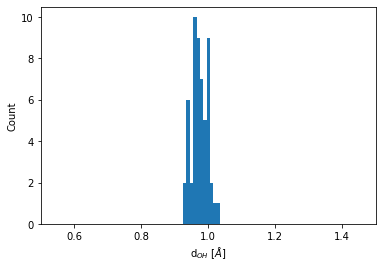
Distribution of the O-H bond length#
Every O atom has two H atoms as immediate neighbors. The distribution of this bond length is obtained by:
bins = np.linspace(0.5, 1.5, 100)
plt.hist(neighbors.distances[O_indices].flatten(), bins=bins)
plt.xlim(0.5, 1.5)
plt.xlabel(r"d$_{OH}$ [$\AA$]")
plt.ylabel("Count");
Distribution of the O-O bond lengths#
We need to extend the analysis to go beyond nearest neighbors. We do this by using the number of neighbors in a specified cutoff distance
num_neighbors = final_struct.get_numbers_of_neighbors_in_sphere(cutoff_radius=9).max()
neighbors = final_struct.get_neighbors(num_neighbors)
neigh_indices = np.hstack(np.array(neighbors.indices)[O_indices])
neigh_distances = np.hstack(np.array(neighbors.distances)[O_indices])
One is often intended in an element specific pair correlation function. To obtain for example, the O-O coordination function, we do the following:
# Getting the neighboring Oxyhen indices
O_neigh_indices = np.isin(neigh_indices, O_indices)
O_neigh_distances = neigh_distances[O_neigh_indices]
bins = np.linspace(1, 8, 120)
count = plt.hist(O_neigh_distances, bins=bins)
plt.xlim(2, 4)
plt.title("O-O pair correlation")
plt.xlabel(r"d$_{OO}$ [$\AA$]")
plt.ylabel("Count");

We now extent our analysis to include statistically independent snapshots along the trajectory. This allows to obtain the radial pair distribution function of O-O distances in the NVT ensamble.
traj = ham_eq["output/generic/positions"]
nsteps = len(traj)
stepincrement = int(nsteps / 10)
# Start sampling snaphots after some equilibration time; do not double count last step.
snapshots = range(stepincrement, nsteps - stepincrement, stepincrement)
for i in snapshots:
    struct.positions = traj[i]
    neighbors = struct.get_neighbors(num_neighbors)
    neigh_indices = np.hstack(np.array(neighbors.indices)[O_indices])
    neigh_distances = np.hstack(np.array(neighbors.distances)[O_indices])
    O_neigh_indices = np.isin(neigh_indices, O_indices)
    # collect all distances in the same array
    O_neigh_distances = np.concatenate(
        (O_neigh_distances, neigh_distances[O_neigh_indices])
    )
To obtain a radial pair distribution function (\(g(r)\)), one has to normalize by the volume of the surfce increment of the sphere (\(4\pi r^2\Delta r\)) and by the number of species, samples, and the number density.
O_gr = np.histogram(O_neigh_distances, bins=bins)
dr = O_gr[1][1] - O_gr[1][0]
normfac = (n / a) ** 3 * n**3 * 4 * np.pi * dr * (len(snapshots) + 1)
# (n/a)**3            number density
# n**3                number of species
# (len(snapshots)+1)  number of samples (we also use final_struct)
plt.bar(O_gr[1][0:-1], O_gr[0] / (normfac * O_gr[1][0:-1] ** 2), dr)
plt.xlim(2, 7)
plt.title("O-O pair correlation")
plt.xlabel(r"d$_{OO}$ [$\AA$]")
plt.ylabel("$g_{OO}(r)$");
